research
overview
Optimization is the computational engine of data science and machine learning. Training a model, matching one data distribution to another, and simulating how a system evolves all come down to minimizing a function. The workhorse algorithms are first-order methods, which use only gradients. They are simple and scale to very large problems, but they slow down dramatically on poorly conditioned problems, which are much steeper in some directions than in others.
Three ideas make these methods fast in practice. Acceleration uses momentum to reach a solution in far fewer steps. Preconditioning, of which mirror descent is one form, changes the geometry of the problem so that it becomes easier to solve. Adaptivity tunes the step size and other parameters during the run, instead of relying on constants that are rarely known in advance. These ideas are usually designed and analyzed one at a time.
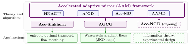
My research develops a single framework that combines all three, which I call the accelerated adaptive mirror (AAM) framework. It views an algorithm as a time-stepping scheme for a continuous-time process, and uses a quantity that decreases along that process, a Lyapunov function, to design the algorithm, choose its parameters, and prove how fast it converges. This turns widely used algorithms into much faster ones that stay as simple as the originals. The main results so far are:
- A unified theory of acceleration, adaptivity, and preconditioning, including AAMD, a method that provably combines all three.
- Acc-Sinkhorn, a faster version of the Sinkhorn algorithm for optimal transport, the standard tool for comparing and matching probability distributions. Each step costs the same as a Sinkhorn step, and the speedup grows on the hardest problems, where Sinkhorn is slowest.
- AGCG, an accelerated method for Wasserstein gradient flows, which describe how a distribution of mass, such as a granular material, evolves over time. As the problem gets harder, its cost grows like the square root of the difficulty, while that of existing adaptive methods grows almost in proportion to it.
- Generative modeling. In recent experiments, Acc-Sinkhorn cut the training time of a class of image-generation models, one-step flow-matching models, by about 30%.
interactive demos
Each topic below opens to a short introduction and an interactive demo.
Acceleration
Consider \(\min_{x \in \mathbb{R}^n} f(x)\), where \(f\) is \(L\)-smooth and \(\mu\)-strongly convex, with condition number \(\kappa = L/\mu\). Gradient descent with step size \(1/L\), $$x_{k+1} = x_k - \tfrac{1}{L} \nabla f(x_k),$$ satisfies \(f(x_k) - f^\star \le (1 - 1/\kappa)^k \, (f(x_0) - f^\star)\). Nesterov's accelerated gradient method adds a momentum step, $$y_k = x_k + \beta (x_k - x_{k-1}), \qquad x_{k+1} = y_k - \tfrac{1}{L} \nabla f(y_k), \qquad \beta = \frac{\sqrt{\kappa} - 1}{\sqrt{\kappa} + 1},$$ and satisfies $$f(x_k) - f^\star \le (1 - 1/\sqrt{\kappa})^k \, \big(f(x_0) - f^\star + \tfrac{\mu}{2} \|x_0 - x^\star\|^2\big).$$ The iteration count to reach accuracy \(\varepsilon\) drops from \(O(\kappa \log(1/\varepsilon))\) to \(O(\sqrt{\kappa} \log(1/\varepsilon))\), which is optimal among first-order methods for this class.
Demo. On \(\mathbb{R}^2\), $$f(x) = \log \sum_i \exp(\langle a_i, x \rangle + c_i) + \tfrac{1}{2}(m_1 x_1^2 + m_2 x_2^2).$$ The \(\kappa\) slider shrinks \(m_1\). \(L\) and \(\mu\) are the extreme Hessian eigenvalues over the plotted region; dashed lines show the two rates. Surface height is \(\sqrt{f - f^\star}\), rescaled, which keeps the level sets. Drag the surface to rotate it; click it to move the starting point.
Mirror descent
Let \(h\) be a differentiable convex reference function with Bregman divergence \(D_h(x, y) = h(x) - h(y) - \langle \nabla h(y), x - y \rangle\). Mirror descent replaces the Euclidean proximity term of gradient descent with \(D_h\): $$x_{k+1} = \arg\min_x \big\{ \langle \nabla f(x_k), x \rangle + L \, D_h(x, x_k) \big\} \quad \Longleftrightarrow \quad \nabla h(x_{k+1}) = \nabla h(x_k) - \tfrac{1}{L} \nabla f(x_k).$$ We say \(f\) is \(L\)-smooth and \(\mu\)-strongly convex relative to \(h\) if $$\mu \, D_h(x, y) \le D_f(x, y) \le L \, D_h(x, y) \quad \text{for all } x, y.$$ Under these conditions mirror descent converges linearly, \(f(x_k) - f^\star = O\big((1 - \mu/L)^k\big)\) (Lu, Freund and Nesterov, 2018). With \(h = \tfrac{1}{2}\|x\|^2\) this is gradient descent. The gain comes when \(\kappa = L/\mu\) relative to \(h\) is far smaller than the Euclidean condition number, or when no Euclidean \(L\) exists at all.
Demo. \(f(x) = \tfrac{1}{4}\|Ex\|^4 + \tfrac{1}{4}\|Ax - b\|_4^4 + \tfrac{1}{2}\|Cx - d\|^2\) and \(h(x) = \tfrac{1}{4}\|x\|^4 + \tfrac{1}{2}\|x\|^2\). The Hessian of \(f\) grows without bound, so \(f\) has no global Euclidean \(L\), but it is smooth and strongly convex relative to \(h\). The mirror step inverts \(\nabla h(x) = (1 + \|x\|^2)\,x\) by solving a cubic in \(\|x\|\). Both condition numbers are measured over the plotted region: Euclidean from the eigenvalues of \(\nabla^2 f\), relative from those of \(\nabla^2 h^{-1/2} \nabla^2 f \, \nabla^2 h^{-1/2}\). The slider scales \(A\). Drag the surface to rotate it; click it to move the starting point.
Adaptivity
Gradient descent with a fixed step \(\eta\) on a quadratic \(f(x) = \tfrac{1}{2} x^\top H x\) scales the component along each eigenvector of \(H\) by \(1 - \eta \lambda_i\). It is therefore stable only for \(0 \lt \eta \lt 2/L\), and the best fixed step \(\eta^\star = 2/(L + \mu)\) gives the contraction factor \(\rho = (\kappa - 1)/(\kappa + 1)\), so \(f(x_k) - f^\star\) decays like \(\rho^{2k}\). Choosing \(\eta\) well requires knowing \(L\) and \(\mu\). Adaptive methods instead set the step from quantities observed during the run:
- Polyak step: \(\displaystyle \eta_k = \frac{f(x_k) - f^\star}{\|\nabla f(x_k)\|^2}\), which needs only \(f^\star\).
- AdaGrad (diagonal): $$G_{k,i} = \sum_{j \le k} \big(\partial_i f(x_j)\big)^2, \qquad x_{k+1,i} = x_{k,i} - \frac{\eta_0}{\sqrt{G_{k,i}} + \epsilon} \, \partial_i f(x_k).$$ Each coordinate gets its own step. This is mirror descent with the data-dependent reference function \(h_k(x) = \tfrac{1}{2} x^\top \operatorname{diag}(\sqrt{G_k}) \, x\).
Demo. \(f(x) = \tfrac{1}{2}(\kappa x_1^2 + x_2^2)\), so \(L = \kappa\) and \(\mu = 1\) exactly. The fixed-step slider has ticks at \(\eta^\star\) and \(2/L\); the dashed line is the optimal fixed-step rate \(\rho^{2k}\). The lower panel shows \(\eta_k\), per coordinate for AdaGrad. Drag the surface to rotate it; click it to move the starting point.